May 13, 2020
General
Acoustic Doppler Current Profilers (ADCP) are hydro-acoustic instruments that are used to measure water velocities or currents over a specific range of water depth. ADCPs utilizes the Doppler effect to measure water velocity in discrete layers – essentially sending a sound signal of a specific frequency into the water column and measuring the sound signal return. The change in return frequency is proportional to the water velocity. ADCPs can be deployed in many ways, up-looking, down-looking, and side-looking. In all cases, velocity data is collected,
but the flexibility in mounting the ADCP allows for novel ways of understanding current information of the site in interest. In addition to measuring velocity, ADCPs can be used to measure distance to the
water surface (for bottom mounted systems) or distance to the bottom for surface,
or subsurface, down-looking systems. Using an ADCP to find the bottom is called
bottom tracking and is often used for navigation. Although the ADCP hardware is
essentially the same, the instrument is configured differently to collect bottom track
data. When used in this manner the instrument is called a DVL, or Doppler Velocity
Log. In DVL mode, the instrument not only collects distance to bottom information,
but can also collect vehicle speed as well as water velocity information. When
combined with additional data, such as, initial position and heading, DVLs can be
used for underwater navigation (AUV, ROV, submarines, etc.).
The following general schematic highlights the various methods of deployment and
applications for ADCPs and DVLs.
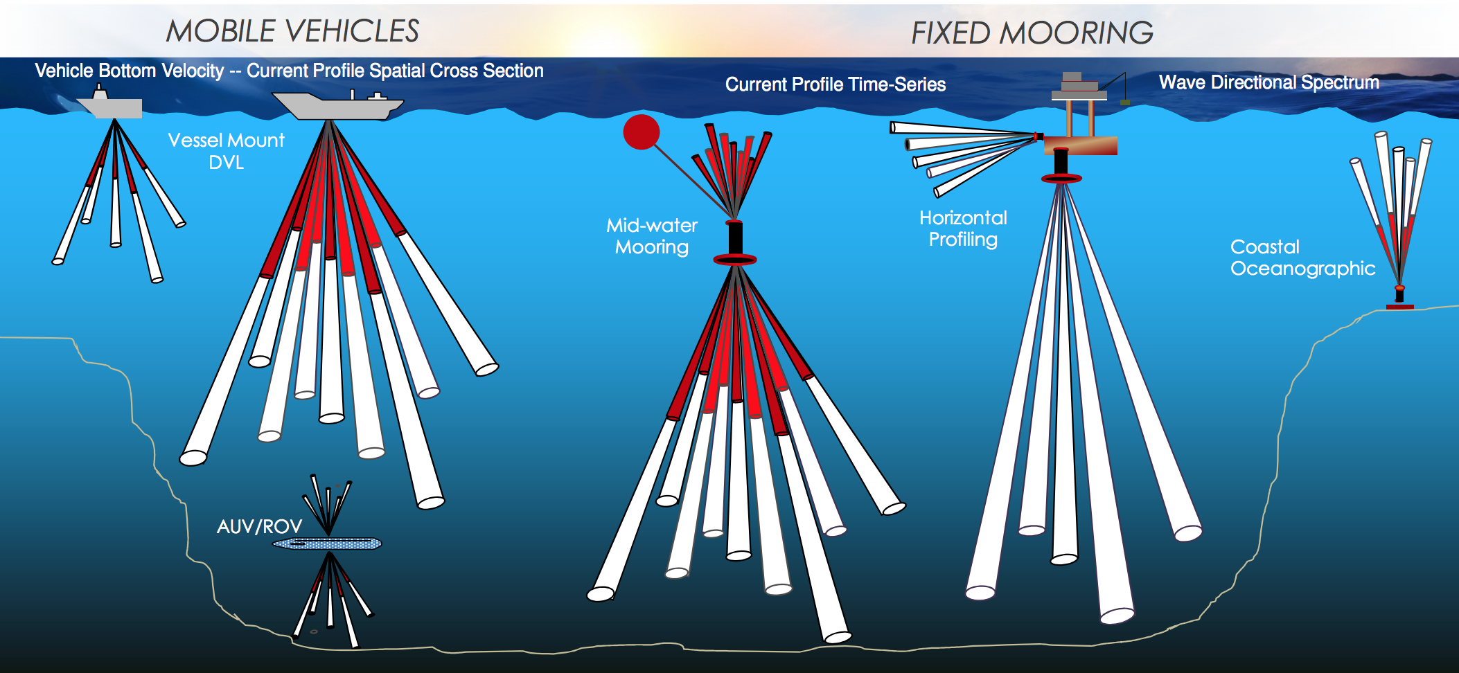
Mobile Vehicle Applications
Mobile vehicle applications utilize ADCPs and DVLs to profile currents and track the sea or river bottom.
Navigation – In DVL mode, the instrument can be used in all sizes of ships, AUVs, and ROVs, but using the instrument’s bottom track capability coupled with instrument heading, pitch and roll information. In addition to tracking the bottom and providing vessel navigation information, the DVL also provides current profiling data. DVLs have been very popular in the AUV market for search and rescue as well as bathymetry studies. DVLs are increasingly used with ROVs for navigational purposes.
Vessel Mount – are systems are used to monitor currents below the ship, and when possible, provide bottom-track information. RTI’s Doppler array systems are the smallest in the industry, minimizing costs for installation and commissioning. Vessel Mount systems have been used to measure currents for climate change and ocean mapping studies, as well as other more specialized research.
Discharge/Flow – utilize an ADCP on a small boat or tethered platform to measure velocity profiles to determine flow or discharge in an open channel (rivers or canals). In this application, flow is determined from bathymetry (bottom track data) and the cross-sectional area of flow, combined with velocity profile information to determine flow rate.
Fixed Position Deployments
Surface moorings (deep water) – typically utilizes an ADCP, up or downlooking, to measure currents. In the case of down-looking systems, the ADCP can be installed at the surface or below the surface. For up-looking systems the ADCP is installed below the surface and measures currents towards the surface.
Subsurface moorings (deep water/up or down-looking) – are typically anchored to the sea floor with a sub-surface buoy supporting a string of instrumentation in the vertical. In this case, ADCPs can be installed up- and down-looking to profile currents in both directions. In addition, downlooking systems can track the bottom and be used for boundary layer studies. Bottom mounts (shallow water) – Bottom mounted systems measure a variety of parameters using an ADCP. Most oceanographic applications systems are up-looking and measure currents and waves (direction and wave height). However, there are some applications where the ADCP is installed on the sea floor and in a down-looking orientation in order to conduct boundary layer studies. For hydrology applications, ADCPs can be mounted on the channel bottom, looking up to measure velocity profiles and water depth. These two pieces of data can used to calculate flow rate (water level combined with area rating determines the area of flow and is multiplied by velocity profile data to determine flow rate).
Side-looking – ADCPs are typically utilized in large channels and in harbors to monitor currents. Flow can be determined by knowing the water level and bathymetry.
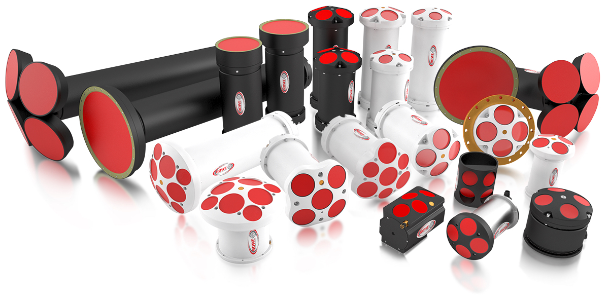
This is a sample of the products that are available from Rowe technologies. It includes a combination of shallow and deep water Doppler Piston products as well as low frequency Planar Array products.
ADCP/DVL Hardware
When considering an ADCP or DVL, it is fundamental to understand how the system will be used and what type of power is available. Direct reading systems are connected to a power source or are integrated into a system that provides power. Self-contained systems are autonomous systems that utilize battery packs to power the instruments.
Rowe Technologies Inc. manufactures ADCPs/DVLs in both the familiar Janus configuration,
which uses multiple, symmetrically spaced “piston” transducers in the ADCP head,
as well as planar array systems that essentially have one transducer or an array of
mini-transducers, all contained in the same small compact instrument head. Planar
array systems, referred to as Doppler Arrays, have the same, or better performance
as piston transducers by generating multiple beams from the planar aperture;
however, the form factor is much smaller. The photo following is a good example of
this. It compares a traditional 300 KHz 4-piston Janus configuration with a 300 KHz
Doppler Array system. Note that the Doppler Array is approximately one-quarter
the size of the Janus head, but offers similar, or better, performance. This size advantage becomes more pronounced as frequencies go lower and acoustic
apertures become larger to maintain performance.
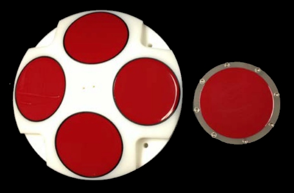
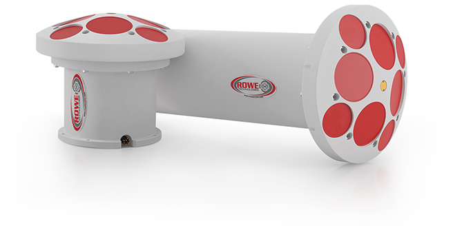
As another example, the image following shows a 300KHz Janus head ADCP (left)
and a 150 KHz Doppler Array (right). Note that although the Doppler Array is
approximately half the frequency, it is roughly the same size, weight and volume as
the 300 KHz system, but the 150 KHz system has twice the profiling range.
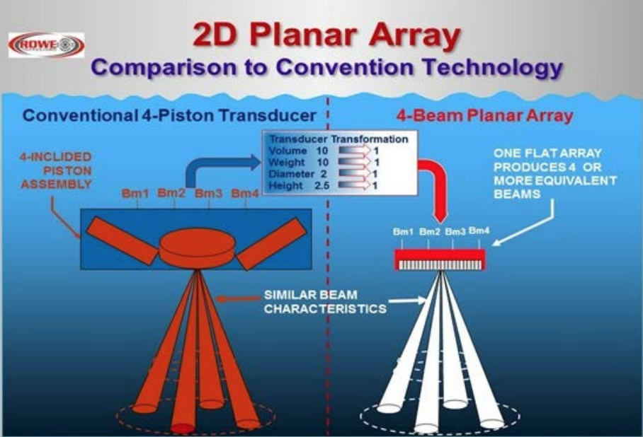
The schematic following highlights the differences in the traditional piston and
planar array systems.
Dual Frequency Systems
Dual Frequency systems are available in both piston and Doppler Array
configurations (see following below). For piston systems (on the left), additional
transducers are embedded in the ADCP head for each frequency. The example
below is for a 1200 KHz and 300 KHz dual frequency system. For dual frequency
Doppler Array systems, there are two independent Doppler Arrays of different
frequencies, assembled in a “doughnut hole” configuration. The center of the array
has a transducer with a frequency that is different than the outer doughnut
transducer (following image on the right).
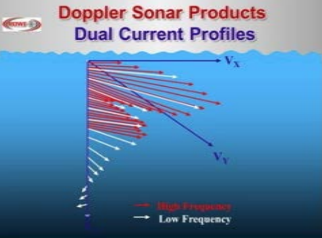
Advantages of Dual Frequencies Systems
Dual Frequency systems combine the attributes of two distinct acoustic frequencies,
combining extended range and high-resolution data and more information about the sampling area. Low frequency systems provide long range and low-resolution
measurements, while high frequency systems have shorter ranges with much higher
resolution. By combining frequencies, ADCP users have the opportunity to collect
long-range and high-resolution data. The following graphic highlights data that can
be collected with dual frequency systems.
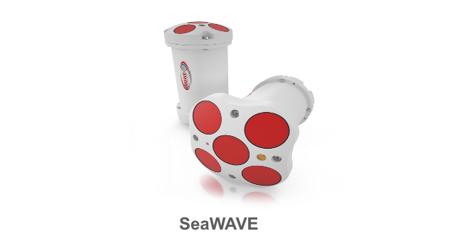
Vertical Beams
The SeaWAVE and SeaSEVEN ADCPs are two new products that use both a vertical
beam and a JANUS beam configuration. The SeaWAVE simultaneously measures
wave spectra, wave direction and complete current profiles for every ping. This
ADCP uses both the vertical beam and a pressure sensor to accurately measure
range to the surface. This vertical beam functions similar to an inverted echo
sounder providing more accurate, higher frequency wave measurements.
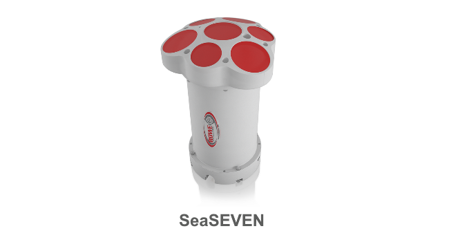
The SeaSEVEN is designed with maximum performance and flexibility for advanced
research, featuring: dual frequency, a vertical beam, high ping
rate/resolution/accuracy, and long range performance with ultimate controllability.
The SeaSEVEN is intended to fill a void in today’s data-rich environment, with a high
capacity data recorder, multi-mission capability, external sensor integration and
ultra-fast Ethernet data download. With its low aperture splayed beam array, and
modern electronics, it provides measurements not available from any other Doppler
Profiler. It collects, stores and transmits the data to allow advanced ocean research
never before seen in a Doppler profiler.
Current Profiling And Bottom Tracking Range
Current profiling and bottom tracking range is a function of acoustic frequency and
beam angles (described in the following table). Depending on the deployment
requirements, RoweTech ADCPs and DVLs offers options for HI and LOW power
transmitting. This option will allow increased range in the case of the HI power
setting and a decreased range but an increased battery life for the LOW power
setting. The table shows achievable ranges for both narrowband and broadband
profling, as well as bottom track ranges, for high power operating mode.
| 75 kHz | 150 kHz | 300 kHz | 600 kHz | 1200 kHz | |
| Current Profile | |||||
| Narrowband | 700m | 425m | 180m | 90m | 30m |
| Broadband | 455m | 275m | 100m | 50m | 20m |
| Bottom Track | 1000m | 700m | 350m | 120m | 50m |
Beam Angles
An important consideration when deploying an ADCP/DVL is beam angle. The beam angle is the angle at which the beam is oriented with respect to the axis normal to the transducer head. This angle directly impacts instrument range - the larger the beam angle, the shorter the range. There is, however, a benefit for a larger beam angle on ADCPs, as there is an improvement in velocity measurements. For most vertical current profiling or bottom-referenced velocity applications, the measured current or bottom velocity magnitude is primarily horizontal or parallel to the transducer face as illustrated in the table. The component of the beam in the direction (θv) of the primary horizontal velocity is:
θv = Sin θ
Piston Systems – RTI piston products utilize a 20° beam angle, with each beam (of the four) offset in azimuth by 90°. All beams are fixed in the piston systems.
Planar Array – utilize optional inclined beam angles (θ) of 30° or 20° relative to the
axis normal to the transducer face, plus a beam at 0° (or vertical beam) are user selectable. The 20° beams are also rotated 45 degrees in the azimuth plane from the
30° beam set.
Practical Beam Angle Example:
For 30° beam angles, θv = Sin 30° = 0.50
For 20° beam angles, θv = Sin 20° = 0.34
Thus, 30° beams have a factor of 1.5 larger angular components in the direction of the primary horizontal velocity being measured. The primary benefit of the beam pointing more in the direction of the horizontal velocity is improved short-term velocity precision and long-term accuracy. The short-term precision is improved by a factor of 1.5, and the long-term accuracy is also significantly improved. The current profile and bottom velocity measurement range is increased by the relative vertical beam angle component of:
Cos 20°/Cos 30° = 0.94⁄0.87 = 1.1 (10% more range near bottom boundary)
The primary differences in ADCP/DVL performance for beam angle selection are illustrated as follows, essentially the shallower beam angle has an improved nearbottom current measurement.
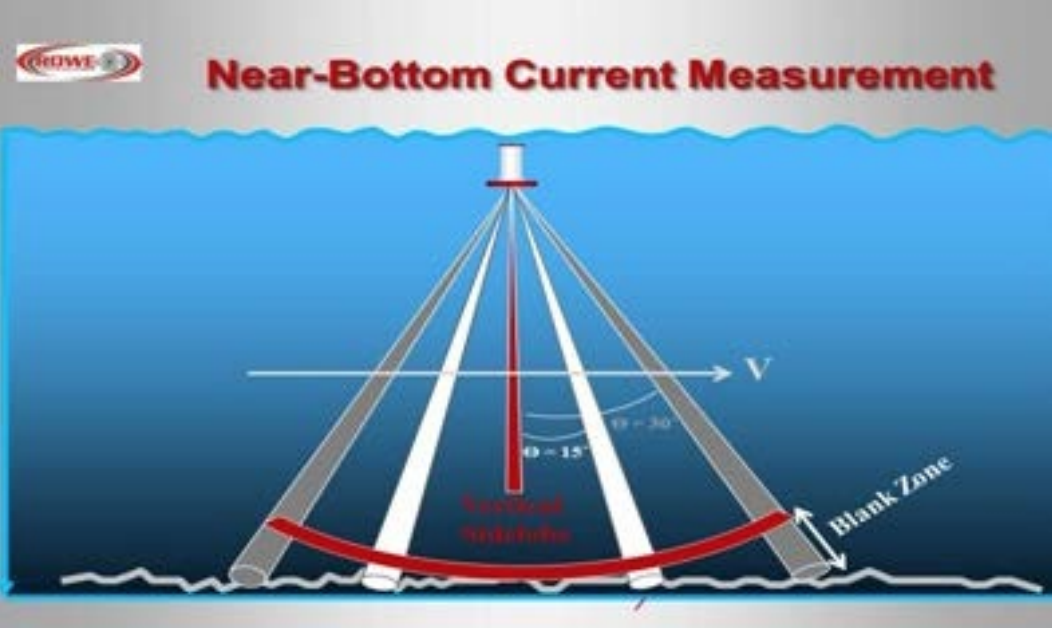
In addition, 20° beam angles improve near bottom current measurements because
vertical side-lobe interference biases the slant range measurements over a nearbottom
range, resulting in a near-bottom “Blank” range as illustrated in the figure.
Blank range = N depth cells + R (1 – Cos θ)
    where R = ADCP/DVL altitude above the bottom
    and N = 1 for Narrowband operation
    and = 2 for Broadband
For example Broadband shallow water application where:
Depth cell = 0.2m and R = 20m
With 30° beam angles, near bottom “blank” range = 0.4m + 0.13(20m) = 2.8m
With 20° beam angles, near bottom “blank” range = 0.4m + 0.06(20m) = 1.3m
By alternating beam angles between 20° and 30°, benefits of 20° beam angle may be achieved, with a degradation of approximately √2 in 30° beam precision in the main water column.
Acoustic Signal Processing
The following an illustration of Broadband and Narrowband operation in the Time,
Space, Frequency, and Autocorrelation domains.
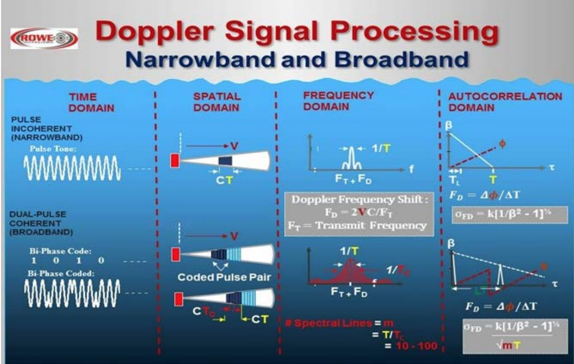
In The Time Domain:
- The Narrowband transmitted pulse is a simple tone burst of time interval (T).
- Broadband transmitted signal is a bi-phase coded pulse pair, where each pulse is of time interval T consisting of m code elements with time delay TC.
In The Underwater Space Domain:
The Narrowband transmitted pulse of length CT propagates along the beam
direction at a velocity of C ± V, where C is the sound speed in water, and V is the
velocity of the transducer relative to the water.
- The dual Broadband transmitted coded pulses, with code element lengths C*TC total length 2CT (For closely spaced pulses) propagates along the beam direction at a velocity of C ± V. At a time delay of T, the 2nd (dark blue) pulse is at approximately the same position along the beam as was the 1st pulse (light blue) at time T earlier. The exact relative position at time delay T differs from CT by T(C±V).
In The Frequency Domain:
- The Narrowband signal of width (1/T) is located at a nominal frequency of FT ± FD, where FT is the transmitted frequency and FD is the Doppler frequency shift = 2VC/FT.
- The Broadband signal of width (1/TC), consisting of m = T/TC spectral lines separated by 1/T, and located at a nominal frequency of FT ± FD.
In The Autocorrelation Domain:
- The Narrowband complex autocorrelation function is centered at zero lag, and decreasing to 0 at Time lag T. The Doppler frequency shift is calculated from the phase shift, Φ, of the autocorrelation function at time lag TL, as FD = Φ/TL. The standard deviation, σFD, of the Doppler frequency calculation is as shown.
- The Broadband complex autocorrelation function has a peak at zero lag and a 2nd narrow peak nominal center at a time lag = Tc. The Doppler frequency shift is calculated from the phase shift, Φ, at the 2nd peak of the of the autocorrelation function, as FD = Φ/TL. The standard deviation, σFD, of the Doppler frequency calculation is as shown. Note that the Broadband σFD is less than the Narrowband by a factor of √mTc.
The Main Conclusions Drawn From The Above Analysis Are:
- The standard deviation of Doppler frequency (and beam radial velocity component) with Broadband operation is lower. For a typical value of m = 16, TC = T, the Broadband to Narrowband Doppler frequency standard deviation reduction factor = √9 = 3.
- The primary advantage of Narrowband is increased signal-to-noise ratio. This is because the Broadband signal spectrum is broader by a factor of T/TC than the Narrowband spectrum, and for matched band processing, the noise bandwidth is correspondingly wider and noise power correspondingly higher. For a fixed transmitted power, the Broadband Signal/Noise power ratio is reduced by a factor of m.
These general conclusions are quantified below showing the Narrowband and Broadband signal-to-noise ratio and velocity measurement standard deviation versus range for an example ADCP operating at an acoustic frequency of 40 kHz, and a fixed size depth cell.
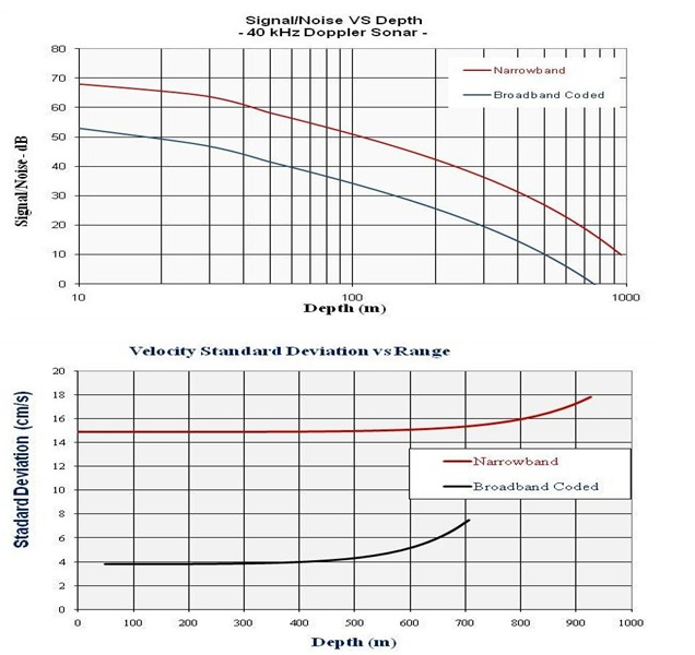
Thus, the primary operational advantage of Narrowband is increased range when compared to Broadband. For Broadband operation the primary advantage is lower velocity standard deviation. This enables increased flexibility in depth, temporal and velocity resolution, when trading off these resolution parameters over a shorter range. Note that this higher precision velocity-performance also results in improved temporal measurement resolution for a fixed ensemble velocity precision, since fewer velocity measurements must be averaged together in an ensemble.
Considering only the velocity noise of the ADCP/DVL, the relationship between the standard deviation of a single-ping velocity measurement (σVP) and the number (N) of pings required to be averaged together to achieve a given Ensemble velocity standard deviation (σVE) is given by: σVE = √N * σVP.
More topics and tutorials can be found at Rowe EDU
For more information about Rowe Technologies ADCPs, please visit:
http://rowetechinc.com/seaprofiler/
sales@rowetechinc.com
+1 (858) 842 3020.